An MLAB Example: The Dynamics of Radioactive Decay

Radioactive decay is a process which occurs at a rate characteristic of the decaying isotope and proportional to the amount of the isotope. The decay process converts the original isotope into a new species called a daughter, which, itself, may also be radioactive and undergo further decay, again at a characteristic rate proportional to the amount of the second isotope, which we may call the granddaughter species. The granddaughter may also be radioactive, but have a non-radioactive decay product. From observation of the time-dependence of the radioactivity of the grand-daughter, we wish to estimate the decay rates of all the three species, and hence, to identify the three isotopes which are involved. This type of identification problem was important, for example, in determining the atomic composition of the star involved in the recently observed supernova.

Denote the amounts of the three isotopes by X, Y, and Z, respectively. Denote the initial amounts of the isotopes by X0, Y0, and Z0; and denote the corresponding rates of decay by K, L, and M, which are positive numbers. The differential equations of the radioactive decay process described above are:

dX/dt = K*X
dY/dt = K*XL*Y
dZ/dt = L*YM*Z

We suppose that only the decay of isotope Z produces radiation which can be detected, and that measurements of radiation from decays of isotope Z (which is proportional to the amount of Z) are made at a series of times Ti, i = 1,2,...,200. These measurements are read into a 200 row, two column matrix called DATA, column 1 of which contains the times, and column 2 of which contains the measured values. We suppose that the initial conditions are known, e.g. X0 = 5000, Y0 = 0, and Z0 = 0. Initial guesses are required for K, L, and M, from which the process of estimating K,L, and M will proceed. We take these guesses to be K=1, L=1, and M=1.

In MLAB, this problem may be formulated as follows:

	* FCT X'T (T) = -K*X
	* FCT Y'T (T) = K*X-L*Y
	* FCT Z'T (T) = L*Y-M*Z
	* INIT X(0) =  5000
	* INIT Y(0) = 0
	* INIT Z(0) = 0
	* K = 1; L = .1; M = .01; 
	* CONSTRAINTS Q = {K > 0, L > 0, M > 0}
	* DATA = READ(DECAY,200,2)

Now we may estimate K, L, and M using the following MLAB FIT statement.

	* FIT (K,L,M),Z TO DATA, CONSTRAINTS Q

The output of the fit statement is the table shown below, containing the least squares estimates, along with standard deviations which help the user to determine the quality of the fit.

	final parameter values
	    value		error          dependency	parameter
	 0.1133576575        0.9382481192     0.9996464477        K
	 0.1171530638        0.8648505987     0.9996463229        L
	 0.01384391436       0.0005651783173  0.07687919473       M
	17 iterations
	CONVERGED
	best weighted sum of squares = 1.315000e+06
	weighted root mean square error = 2.564176e+02
	weighted deviation fraction = 9.784715e-02
	R squared = 9.595270e-01
	no active constraints

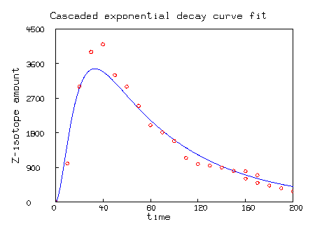
A graph of the data and the fitted curve is a useful measure of the quality of the fit. This is easily done in MLAB.

	* DRAW DATA LINETYPE NONE, PT CIRCLE, PTSIZE 0.01, COLOR RED
	* DRAW POINTS(Z,0:200!160) COLOR BLUE
	* IMAGE COLOR GREY
	* BOTTOM TITLE "time"
	* LEFT TITLE "Z-isotope amount"
	* TOP TITLE "Cascaded exponential decay curve fit"
	* VIEW

MLAB is unique in its power and ease of use in handling differential equations in curve-fitting. Delays, implicitly-defined functions, and recursively-defined functions may all be used. The MLAB differential equation solver uses Adams' fourth order predictor-corrector method for speed and Gear's implicit predictor-corrector method for stiff equations. The derivatives needed for the elements of the Jacobian in Gear's method are computed symbolically and evaluated from the resulting formulas. Integration step size is chosen automatically and varied so as to maximize speed while maintaining specified accuracy.

Send comments to: webmaster@civilized.com