Ultracentrifuge Data Analysis

One common application of curve-fitting occurs in the analysis of ultracentrifuge data. One of the most common uses of an ultracentrifuge is for molecular weight determination. Suppose we load the cell (a wedge-like container with circular-profile surfaces at each end) of an ultracentrifuge with a solution of a substance with an unknown molecular weight, and then spin the cell until the molecules in solution distribute themselves in the cell according to the forces that act upon them. This equilibrium arrangement will have the solute distributed in the cell in an exponential fashion with relatively more of the solute at the bottom (which is the outer end) of the cell. Therefore the concentration of the solute varies at different positions along the cell ( i.e., at different radial positions or distances from the center of the ultracentrifuge.)

Let us denote a given radial position by $r$, measured in centimeters from the center of rotation, where the cell ranges from the top position at $r$_m to the bottom position at the outer end of the cell at $r$_b. Then the concentration of the solute, $c$, measured in grams per liter, at the radial position $r$ is a function of $r$ given as:

$c$_h is the concentration in grams per liter of the solute at a given reference radial position, $r$_h. The value $c$_h can be computed from $N$ and $c$₀the total amount of solute in the cell measured in grams per liter, however, in practice, $c$_h can be determined by curve-fitting.

$r$_h is the given radial reference position (it is not necessary that $r$_h be $r$_b or $r$_m, indeed $r$_b is generally a poor choice).

$N$ is the apparent molecular weight of the solute.

$A$ is a certain constant, defined as: $(1-vp)w2/(2RT)$ where $v$ is the partial specific volume of the solute ($1/v$ is the density of the anhydrous solute, so $v$ is measured in cm$3$/gram), $p$ is the solution density in grams/cm$3$$w$ is the angular velocity of the rotor in radians per second, $R$ is the gas constant ($aproximately\; 8.314\; ·\; 107$ ergs/degree/mole), and $T$ is the absolute temperature.

Due to the non-ideal diffusion behavior of most materials, the observable or apparent molecular weight $N$, at a given radial position $r$, is approximately the following non-linear function of the actual molecular weight, $M:\; N$ approximately equals $M/(1+BMc(r))$ where the parameter $B$ is the so-called virial coefficient, with B > 0.

Thus $N$ is a function of $r$, and we have:

The notation $root(x,a,b,f(x))$denotes a value, $x$₀in the interval $[a,b]$ which is a root of the expression $f(x)$ i.e., $x$₀ is a value such that $f(x$₀) = 0 MLAB provides the root operator as a built-in function ROOT. The value $c$_max is any value greater than $c(r$_b) which is an upper bound for $c(r)$

Now, if we measure the concentration distribution with a UV scanner or with a Rayleigh interferometer attached to the ultracentrifuge and express the results as a table of points $(r$_i,c_i) which gives the observed concentration $c$_iat the radial position $r$_iin the cell, then the root-form equation for $c(r)$given above can be used as a model to fit these points. In this way, $M$can be determined by curve-fitting. The virial coefficient $B$ is also generally treated as a fitting parameter. Often $c$_h is not exactly known, and can also be a fitting parameter. Concentration can be measured in any of a number of different units. Fundamentally, we have fringe numbers or optical densities, and such observations are readily convertible by scaling to grams-per-liter concentration units.

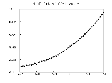
Here is an example showing how the fit is done in MLAB. We first define the model, and then read-in some data, set initial-guess values of the parameters to be fitted, and fit the model to the given data. Finally, we draw pictures of the data and the fitted model.

fct c(r)=root(x, 0.5,20,(ch*exp(A*M*(r^2-rh^2)/(1+M*B*x))-x)) 
data = read(centri,51,2) /* read in the data from file centri.dat */

q = 0.26 /* this term is 1-zbar*rho */
omega = 1047.2 /* corresponding to 10000 rpm machine rotation */
R = 8.314*10^7 /* gas concentration */
t = 298.15 /* absolute temprature */
A = (q*omega^2)/(2*R*t); /* A = 5.75119093E-6 */
rh = 6.7   /* reference radius in cm */

/* set initial guesses for B, ch, M */
B = 10^(-7) 
ch = 1.25; 
M = 60000

fit(M,B,ch), c to data

final parameter values
      value               error                dependency    parameter
 68743.0466061385      1414.898785691          0.9928704243   M
 2.283270139e-07      1.901124729e-08          0.9729368851   B
   0.9799669867        0.0201841151          0.9789628624   ch
4 iterations
CONVERGED
best weighted sum of squares = 3.946440e-01
weighted root mean square error = 9.067387e-02
weighted deviation fraction = 9.884748e-03
R squared = 9.989925e-01

draw data, lt none, pt star, ptsize 0.01
draw points(c,(data col 1))
top title "MLAB fit of C(r) vs. r"
view

Note that our model $c(r)$ is an implicit function. One of the features of MLAB is the ability to handle such models. The MLAB curve-fitting process involves computing the derivatives of $c$ with respect to $B,\; M$and $c$_h. Here are the derivative functions generated by MLAB. When differentiating an implicit function, MLAB makes use of the eval operator defined so that $eval(x,E,F)$denotes the value of the expression $F$ with the value $E$substituted for $x$ within $F$

* type c'B
FUNCTION c'B(r) = EVAL(x,ROOT(x,0.5,20,ch*EXP((A*M*(r^2-rh^2)/(1+M*B*x))-x),
-(((M*x*A*M*(r^2-rh^2))/((1+M*B*x)*(1+M*B*x)))*EXP((A*M*(r^2-rh^2))
/(1+M*B*x))*ch)/(((M*B*A*M*(r^2-rh^2))/((1+M*B*x)*(1+M*B*x)))
*EXP((A*M*(r^2-rh^2))/(1+M*B*x))*ch+1))
* 
* type c'M
FUNCTION c'M(r) = EVAL(x,ROOT(x,0.5,20,ch*EXP((A*M*(r^2-rh^2))/(1+M*B*x))-x),
(((A*(r^2-rh^2)*(1+M*B*x)-B*x*A*M*(r^2-rh^2))/((1+M*B*x)*(1+M*B*x)))
*EXP((A*M*(r^2-rh^2))/(1+M*B*x))*ch)/(((M*B*A*M*(r^2-rh^2))
/((1+M*B*x)*(1+M*B*x)))*EXP((A*M*(r^2-rh^2))/(1+M*B*x))*ch+1))
* 
* type c'ch
FUNCTION c'ch(r) = EVAL(x,ROOT(x,0.5,20,ch*EXP((A*M*(r^2-rh^2))/(1+M*B*x))-x),
EXP((A*M*(r^2-rh^2))/(1+M*B*x))/(((M*B*A*M*(r^2-rh^2))/((1+M*B*x)*(1+M*B*x)))
*EXP((A*M*(r^2-rh^2))/(1+M*B*x))*ch+1))

If we have several solutes with unknown molecular weights, then the equation for the combined concentration distribution is merely the sum of the separate concentration distributions. Thus, curve-fitting can be used to determine several molecular weights simultaneously.

In general, we have: $c(r)\; =\; c$₁(r) + c₂(r) +... + c_n(r) where the concentration of the $i$th solute is $c$_i(r) = c_hi exp(A_i N_i(r²-r_h²)) $N$_i is the apparent molecular weight of the $i$th solute, and $c$_hi is the grams per liter concentration of the $i$th solute at the reference position $r$_h, and $A$_i is the usual constant $(1-vp)w2/(2RT)$described above, particularized for the $i$th solute.

As before, $N$_i is a function of $r$ and the true molecular weight, $M$_i namely: $N$_i approximately equals $M$_i/(1+B_iM_i c(r)) In fact this is an approximation to the relationship:

Usually assuming each value $B$_ik1 is the same, namely $B$_i/n for $1$< k < n and $B$_ikj = 0 for is adequate, and this results in the simple form used above.

Suppose, for example, we have two solutes with molecular weights $M$₁ and $M$₂ Then

It is often of interest to compute the amounts of each component present in the ultracentrifuge cell directly from the gram-per-liter concentration profile function. This can be done by using the equation:

MLAB can be used to compute the equilibrium constant $K$ for the simple binding reaction occurring within the ultracentrifuge cell in many cases.

Let $c$₁(r)denote the grams-per-liter concentration of the first solute substance $X$at radial position $r$, let $c$₂(r)denote the grams-per-liter concentration of the second solute substance $Y$at radial position $r$, and let $c$₃(r)denote the grams-per-liter concentration of the composite third solute substance $Z$ at radial position $r$. Then the combined concentration distribution function is $c(r)\; =\; c$₁(r) + c₂(r) + c₃(r) where the grams-per-liter concentration distribution of the $i$th solute is $c$_i(r) = c_hi exp(A_i N_i(r²-r_h²)) for $i=1,2,3$ .$$

Also, at any fixed radial position $r$, the stochiometric relationship $K=((c$₃(r))/(M₃))/ (((c₁(r))/(M₁))((c₂(r))/(M₂)) holds, where $M$_idenotes the molecular weight of solute $i$ for $i=1,2,3$ Note that $M$₃=M₁+M₂ Thus,

Let $g$_i(r,x):=c_hi exp(A_i M_i(r²-r_h²)/(1+B_iM_ix)) for $i=1,2,3$ Note $g$_i(r,c(r))=c_i(r) Now define $f(c$₁,c₂):=c₁+c₂+Kc₁c₂(M₁+M₂)/(M₁M₂) Then, $c(r)=root(x,0,c$_max,f(g₁(r,x),g₂(r,x))-x) where $c$_max satisfies $c$_max>max_r c(r). We thus have an implicit model for the $c$ vs. $r$ data corresponding to the simple binding reaction occurring in the ultracentrifuge cell. The potentially-unknown parameters of this model are $c$_1h$c$_2h$M$₁$M$₂$B$₁$B$₂ $A$₁$A$₂and $K$ MLAB curve-fitting may now in principle be employed to estimate these parameters. In the case of a self-associative dimerization reaction, this model simplifies with $c$_1h=c_2h$M$₁=M₂$A$₁=A₂and $B$₁=B₂

Generally we cannot successfully estimate the equilibrium constant $K$ when $K$ is small (say ) because our model tends to become increasingly ill-conditioned as $K$decreases. The exact limit depends on the molecular weights, the initially-loaded amounts, and the virial coeficients of the reactants.

There are several more ``rules of thumb'' that we should remember when estimating the equlibrium constant $K$

1. The molecular weights $M$₁and $M$₂should be predetermined and should not be fitting parameters. Any of a number of methods can be used to determine $M$₁and $M$₂; if sequence composition information is known, of course, it should be used to compute the corresponding molecular weight exactly. Similarly, the virial coefficients $B$₁and $B$₂should likewise be predetermined, if possible. (Note that once we have obtained $M$₁$M$₂$B$₁$B$₂ $c$_1hand $c$_2h we can subtract $c$₁(r)+c₂(r)from our data, and then fit $g$₃to the result in order to estimate $B$₃and $c$_3hif this is desired.)

2. The value $c$_maxshould be as small as possible so as to minimize the occurrence of overflows in the derivatives of $c$. This implies that relatively dilute solutions of the reactants should be used. On the other hand, we need to produce an adequate amount of $Z$ material to be represented in the $c(r)$-data. The speed of the ultracentrifuge should be chosen to obtain a distribution of mass which is neither too ``flat'' nor too ``sharp'', i.e., material should not ``pile-up'' at the bottom of the cell. It may sometimes be convenient to discard the data for radial positions near the bottom of the cell in order to be able to reduce the value of $c$_max It is generally wise to discard the data near the bottom of cell in any event because the error in measuring mass concentration is large near the boundary of the cell.

3. It is generally useful to replace $K$by $exp(L)$ where $L=log(K)$and then fit to estimate $L$ This does not generally provide a more exact estimate of $K$but the normal theory standard errors computed for $L$are more likely to be meaningful than are the same quantities for $K$ when estimated directly.

Here is an example of using MLAB to estimate the equilibrium constant for a simple binding reaction. Note we have also used the conservation-of-mass relations for substance 1 (X) and for substance 2 (Y). Choosing parameters to fit the computed masses of X and Y to the known initially-loaded masses is a valuable device to improve our parameter estimates. This can only be done, however, when accurate values of $v$ and $r$_b are available. (Another device that can help in obtaining more accurate estimates is to simultaneously fit gram-per-liter concentration-profile data obtained at equilibrium for several different rotor speeds.)

* rm = 6.7  /* minimum radius in cm */
* rb = 7.2  /* maximum radius in cm */
* rh = rm   /* reference radius in cm */
* vc = 2*asin(.33/(2*rb))  /*angle of the cell wedge */
* vc=vc*1.2 /*volume constant, total solution vol.= (vc/2)*(rb^2-rm^2) cm^3 */
 
* r1 = rm:rb:.01 /* radial positions for curve-plotting */
 
* qv = 0.26 /* this term is 1 - zbar*rho */
* omega = 1047.2 /* corresponding to 10000 rpm machine rotation */
* R = 8.314*10^7 /* gas concentration */
* t = 298.15 /* absolute temperature */
* A1 = (qv*omega^2)/(2*R*t); A2 = A1 /* Both A1 and A2 = 5.75119093E-6 */

* /* predetermined values for known parameters */
* B1 = 2*10^(-8); B2=10^(-9);
* M1 = 67000;  M2=6800

 
 
* constraints q={90, ch2>0, ch1+ch2<1.4}
 
* fct g1(r,x)=ch1*exp(A1*M1*(r^2-rh^2)/(1+M1*B1*x))
* fct g2(r,x)=ch2*exp(A2*M2*(r^2-rh^2)/(1+M2*B2*x))
* fct f(c1,c2)=c1+c2+exp(lk)*c1*c2*(M1+M2)/(M1*M2)
* fct c(r) = root(x,(ch1+ch2)/3,100000, f(g1(r,x),g2(r,x))-x)
 
* fct c1(r)=g1(r,c(r))
* fct c2(r)=g2(r,c(r))
* fct c3(r)=c3h(r,c(r))
* fct c3h(r,x)=x-g1(r,x)-g2(r,x)
 
* /*tm1, tm2  = total mass in grams of substances 1 and 2 */
* fct tm1()=integral(r,rm,rb,tm1z(r,c(r))*vc*r)
* fct tm1f(c1,c2,c)=c1+(M1/(M1+M2))*(c-c1-c2)
* fct tm1z(r,x) = tm1f(g1(r,x),g2(r,x),x)
 
* fct tm2()=integral(r,rm,rb,tm2z(r,c(r))*vc*r)
* fct tm2f(c1,c2,c)=c2+(M2/(M1+M2))*(c-c1-c2)
* fct tm2z(r,x) = tm2f(g1(r,x),g2(r,x),x)
 
* /*specify the total mass in grams of substances 1 and 2 */
* mass1[1]= .113689839;
* mass2[1]= .00613855051
 
* /* read-in the r vs. c(r) data to be modeled. */
* data = read(data.dat,1000,2)
* n=nrows(data);
* 
* /* define the weights for fitting and normalize them to sum to 1 */
* zw=ewt(data); zw=zw/rowsum(zw)
 
* /*set initial guesses for k, ch1,and ch2 */
* k=10000; lk=log(k)
* ch1=.15;
* ch2=.035
 
* fit(lk,ch1,ch2), c to data with weight zw, tm1 to mass1, tm2 to mass2,\
: constraints q

 final parameter values
      value               error                dependency    parameter
 10.92859862         0.1533653124            0.9980490348   LK
  0.09847696449      0.003231742687          0.9986427864   CH1
  0.01982622037      0.001226384415          0.9914474897   CH2
4 iterations
CONVERGED
best weighted sum of squares = 2.386287e-05
weighted root mean square error = 6.908382e-04
weighted deviation fraction = 5.217909e-03
R squared = 9.998792e-01
no active constraints

* exp(lk)  /* k=exp(lk) */
    = 55748.1007
* tm1()    /* estimated total mass in grams of X */
    = .113740813
* tm2()    /* estimated total mass in grams of Y */
    = 6.25476406E-3

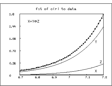
* draw data, lt none, pt star, ptsize 0.01
* draw points(c,r1)
* top title "fit of c(r) to data"
* draw points(c1,r1), color red
* draw points(c2,r1), color green
* draw points(c3,r1), color yellow
* title "Y" at (7.15,.95) world
* title "Z" at (7.18,.36) world
* title "X" at (7.15,.095) world
* title "X+Y'2T='RZ" at (6.75,1.55) world
* view

When we have self-associating molecules in an ultracentrifuge that self-associate in a more complex manner than simple dimer formation, we can still determine the monomer molecular weight, and the equilibrium constants of the known association reactions by curve-fitting in MLAB.

For example, suppose we have the self-associating reactions:

If we let these reactions take place in an ultracentrifuge cell, and measure the weight-average molecular weight, $M$_wof the resulting mixture in grams for different values of $c$, the total concentration in grams per liter of all the species $c$₁, $c$₂, $c$₄and $c$₈ then we can simultaneously determine the monomer molecular weight of the species $c$₁: $M$₁and the equilibrium constants $K$₁₂ $K$₂₄$K$₄₈by curve-fitting.

We have $M$_w = (c₁M₁+c₂M₂+c₄M₄+c₈M₈)/c where $M$_i is the molecular weight of $c$_iand the symbol $c$_ias a function, denotes the gram-per-liter equilibrium concentration of the species $c$_i c is the total gram-per-liter concentration, so $c\; =\; c$₁+c₂+c₄+c₈

Note that $M$₂ = 2M₁$M$₄ = 4M₁and $M$₈ = 8M₁ Also,

Thus, the corresponding equilibrium constants for gram-per-liter concentrations can be defined as:

Define $E$₁₄ = E₂₄E₁₂²and $E$₁₈ = E₄₈E₂₄²E₁₂⁴

Now, $c\; =\; c$₁+c₂+c₄+c₈so $c\; =\; c$₁+E₁₂c₁²+E₁₄c₁⁴+E₁₈c₁⁸ and thus, $c$₁ = root(x,0,c,(x+E₁₂x²+E₁₄x⁴+E₁₈x⁸-c))

Also, $M$_w = M₁(c₁+2E₁₂c₁²+4E₁₄c₁⁴+8E₁₈c₁⁸)/c

Due to the non-ideal gas behavior of most materials, the observed weight-average molecular weight $N$ is, in fact, more nearly the following non-linear function of the actual weight-average molecular weight: $N\; =M$_w/(1+BM_wc) where the parameter $B$ is the so-called virial coefficient.

Thus, given data: $c$ vs.\ $N$, we can fit for the parameters $E$₁₂$E$₂₄$E$₄₈$B$and $M$₁in the following model, as defined in MLAB.

*FUNCTION MA(C) = NID(C,M1*MWX(C,E12,E14,E18),B)
*FUNCTION NID(C,MW,B) = MW/(1+B*C*MW)
*FUNCTION MWX(C,A1,A2,A3) = P(C1(C,A1,A2,A3),A1,A2,A3)/C
*FUNCTION P(C1,A1,A2,A3) = C1+2*A1*C1^2+4*A2*C1^4+8*A3*C1^8
*FUNCTION C1(C,A1,A2,A3) = ROOT(X,0,C,X+A1*X^2+A2*X^4+A3*X^8-C)

In order to obtain the data $c$ vs.\ $N$, preliminary analysis of the actual observations is required. What is, in fact, observed is $r$ vs.\ $c$, where $r$ is a radial position in the cell and where the total gram-per-liter concentration $c$ is observed as a function of $r$. We have the fundamental relation: $c(r)\; =\; c$_hexp(AN(r²-r_h²)), where $A$, $c$_h, and $r$_h are defined above.

Now one can take a few neighboring observations, say five points $(r$₁,c(r₁))$(r$₂, c(r₂))..., $(r$₅, c(r₅)) and fit the above equation to these points with $c$_h = c(r₃)and $r$_h = r₃and thus determine the value of $N$ which corresponds to $c(r$₃) Sliding this operation over all the observations transforms the data so that the model above for $c$ vs.\ $N$ data is now applicable.

Alternatively, one may use the $r$ vs.\ $c$ observations directly by using an implicit model based on the following equations.

In MLAB we have:

*FUNCTION C(R) = P(C1(R,B,M1,C1H),E12,E14,E18)
*FUNCTION P(X,A1,A2,A3) = X+A1*X^2+A2*X^4+A3*X^8
*FCT C1(R,B,M1,CH1) = ROOT(Y,0,MAXC1,Y-CH1*EXP(A*(R*R-RH*RH)*M1/(1+B*M1*Y)))

Although using this model to fit $r$ vs.\ $c$ data to obtain the parameters $B$$M$₁$E$₁₂ $E$₁₄$E$₁₈and possibly $c$_h1 is probably more accurate than the indirect method above, it has the disadvantage that when, as is common, different experiments with different $c$_h1values (and perhaps different $A$ values) are used to cover a wider range of $c$ values, then a curve-fit involving several models being fit simultaneously to adjust shared parameters must be employed, and this is impractical when too many experiments are involved.

In either case, $K$₁₂$K$₂₄and $K$₄₈can then be determined from $E$₁₂$E$₁₄$E$₁₈and $M$₁ Similar models can be obtained for many other specific forms of self-association. The special case where all possible species can arise due to sequential binding, with each binding requiring the same change of free energy as any other is discussed below.

Suppose we have a non-specific isodesmic ``stacking'' reaction involving a monomer $c$₁.

An isodesmic association is one where the free energy for adding one more monomer, $c$₁, to an oligomer, $c$_n, is the same for all $n$.

As before, let $c$_ialso denote the number of grams-per-liter of the species $c$_iin the cell at equilibrium, thus $c$_i is the grams-per-liter concentration of the identically-named species. Also let $c\; =\; c$₁+c₂+...and $M$_w = (c₁M₁+c₂M₂+...)/c where $M$_i is the molecular weight of the species $c$_i; thus $c$ is the total grams-per-liter concentration of all species present, and $M$_w is the weight-average molecular weight of all species.

Now, $K\; =\; (c$_i+1/M_i+1)/((c₁/M₁)(c_i/M_i))so $c$_i+1/M_i+1 = K(c₁/M₁)(c_i/M_i)and hence by successive substitution $c$_i+1/M_i+1 = K_i(c₁/M₁)ⁱ⁺¹

Thus $c$_i = i(K/M₁)^i-1c₁ⁱand hence $c\; =\; c$₁(1+2Kc₁/M₁ + 3(Kc₁/M₁)² +...) But $1+2x+3x2+...\; =\; 1/(1-x)2$so $c\; =\; c$₁/(1-Kc₁/M₁)² where $K$ is the molar equilibrium constant, subject to the constraint that $Kc$₁/M₁ < 1

Also, $M$_w = (M₁c₁+2M₁(2(Kc₁/M₁)c₁)+3M₁(3(Kc₁/M₁)2c₁)+...)/cso $M$_w = c₁M₁(1+ 2²(Kc₁/M₁)+3²(Kc1/M1)2+...)/c; and $12+22x+32x2+...\; =\; (1+x)/(1-x)3$so $M$_w = c₁M₁(1+Kc₁/M₁)/(1-Kc₁/M₁)³/c. Substituting $c$₁/(1-Kc₁/M₁)² for $c$, we have $M$_w = M₁(M₁+Kc₁)/(M₁-Kc₁)

Now, $c$₁ is the function of c given by $c$₁(c) = root(x,0,c,x/(1-Kx/M₁)²-c)and in terms of this function $M$_w = M₁(M₁+Kc₁(c))/(M₁-Kc₁(c)) As before the apparent weight-average molecular weight $N$_w is approximately given by $M$_w/(1+BM_wc)so we may use the model % $N$_w(c) = M₁/((M₁-Kc₁(c))/(M₁+Kc₁(c))+BM₁c) % to fit $c$ vs. $N$_wdata.

Also, since $c(r)\; =\; c$_hexp(AN_w(r₂-r_h²)) we can use the model % $c(r)\; =\; root(x,0,c$_max,(x - c_hexp(AN_w(x)(r₂-r_h²))) % to fit $r$ vs.\ $c$ data.

The equations above are examples of the type of models involved in the analysis of data obtained from the use of an ultracentrifuge. There are many other useful experiments, with other equations (or differential equations) describing the phenomena involved. A good reference on the use of the ultracentrifuge and the associated mathematical modeling is the chapter by K.E.\ Van Holde in the book The Proteins, 3rd edition, Vol.~1, 1975. Another source is {\em Foundations of Ultracentrifugical Analysis}, by Hiroshi Fujita, Wiley, 1975.