Suppose we have an infectious disease agent which infects a susceptible individual and remains untransmittable by that individual for a latent time period q. Such an infected individual will be called a latent individual. After q days, a latent individual becomes an infective individual and can transmit the disease to susceptibles. An infective individual also becomes vulnerable to an increased death risk. The death rate for non-infectives is u percent per day, but for infectives, the death rate is (u+a) percent per day. Finally, after a time period of p days, an infective who survives becomes an immune individual, who cannot transmit the disease, and whose risk of death drops back to the population death rate u.

Suppose also that the birth rate is b percent per day. We may define the following functions.

S(t) = the number of suceptible individuals at time t. L(t) = the number of latent infected individuals at time t. F(t) = the number of infective individuals at time t. I(t) = the number of immune individuals at time t.

Now, of the individuals, say D(t) of them, who enter the latent state at time t, D(t)(1-e^-uq) will die during the time period q, so that D(t)e^-uq individuals will enter the infective state at time t+q. Similarly, of the individuals, say E(t) of them,who enter the infective state at time t, E(t)e^-(u+a)p will survive to enter the immune state at time t+p.

Let c be the mean number of susceptible individuals contacted by an individual per day; c might be about .2. Let h be the probability that a contact of a suceptible with an infective results in transmission of the disease. The probability that a contact at time t is with an infective is, of course, F/(S+L+F+I).

To begin, we will "infuse'' our population with F0 newly-arriving infectives over one day, as indicated by the infusion rate function, R, given below. Let

R(t) = if 1 > t and t > 0 then F0 else 0, D(t) = if t < 0 then 0 else chF(t)/(S(t)+L(t)+F(t)+I(t))S(t), E(t) = D(t-q)e-uq,   and G(t) = (E(t-p)+R(t-p))e-(u+a)p.

Thus we have the following differential equations:

dS/dt = b(S+L+F+I) -uS -D(t), dL/dt = D(t) -uL -E(t), dF/dt = R(t)+E(t) -(u+a)F -G(t),   and dI/dt = G(t) -uI,

where S(0) = S0, L(0) = 0, F(0) = 0, and I(0) = 0.

The latency and infective periods lead to delay terms in the differential equations. MLAB deals with delay by linearly interpolating in the table of previous results. Thus, the time interval between requested answer points should be less than min(p/2,q/2) to allow the backward interpolation to apply.

It is interesting to experiment with values for c, h, a, p, q, and F0 to see under what circumstances a disease will die out, oscillate, or infect the entire population. One can replace the factor chF/(S+L+F+I) with a more abstract constant, k, when the disease is not transmitted by contact alone. Also note that epidemiological data can be fit with these equations and the values of a, q, p, h and/or F0 can thus be estimated.

For more material on such models, see: "The mathematical theory of infectious diseases and its applications'', by N.T.J.Bailey, published in 1975 by Charles Griffin in London.

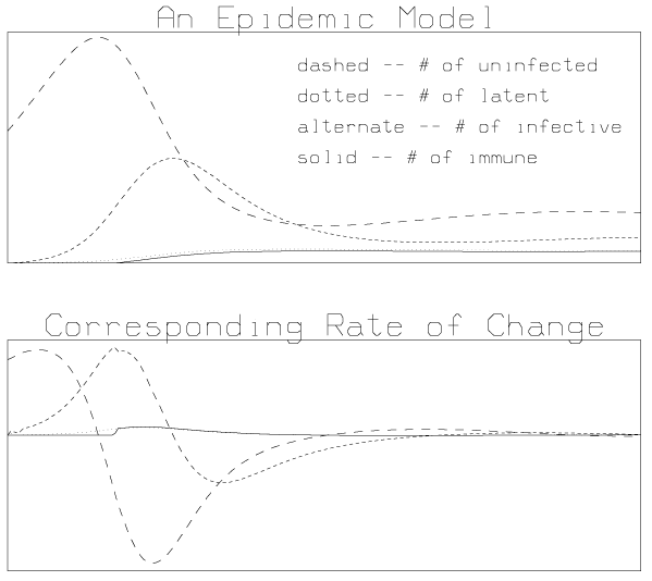
An example using MLAB which results in a new equilibrium being obtained from an initial perturbation is presented below.

"define the epidemic differential equations" 
fct S't(t) = b * (S(t) + L(t) + F(t) + I(t)) - u * S(t) - D(t) 
fct L't(t) = D(t) - u * L(t) - E(t) 
fct F't(t) = R(t) + E(t) - (u+a) * F(t) - G(t) 
fct I't(t) = G(t) - u * I(t)

"define ancillary functions (note the delay)" 
fct R(t) = if (t < t0 and t > 0) then f0 else 0 
fct D(t) = if t < 0 then 0 else c*h*S(t)*F(t)/(S(t) + L(t) + F(t) + I(t)) 
fct E(t) = D(t-q) * exp(-u*q) 
fct G(t) = (E(t-p) + R(t-p)) * exp(-(u+a)*p)

"define system constants" 
f0 = 0.3; s0 = 200; c = 0.5; h = 0.5; p = 30; q = 4; 
u = 0.0072; a = 0.11; b = 0.035; t0 = 40;

"define the initial values" 
init S(0) = s0; init L(0) = 0; 
init F(0) = 0; init I(0) = 0 
"integrate the ODEs" 
M = integrate(S't, L't, F't, I't, 0:200)

frame 0 to 1, .5 to 1 in w1

"graph the number of susceptibles, S(t)" 
draw M col (1,2), linetype dashed, in w1

"graph the number of latents, L(t)" 
draw M col (1,4), linetype dotted, in w1

"graph the number of infectives, F(t)" 
draw M col (1,6), linetype alternate, in w1

"graph the number of immunes, I(t)" 
draw M col (1, 8) linetype solid, in w1

top title "An Epidemic Model", size 0.025, in w1 
title "dashed - # of uninfected", size 0.015, at (.47,.75), in w1 
title "dotted - # of latent", size 0.015, at (.47,.65), in w1 
title "alternate - # of infective", size 0.015, at (.47,.55), in w1 
title "Solid - # of immune", size 0.015, at (.47,.45), in w1

frame 0 to 1, 0 to .5 in w2

"graph the derivative of the number of susceptibles, S't(t)" 
draw M col (1,3), linetype dashed, in w2

"graph the derivative of the number of latents, L't(t)" 
draw M col (1,5), linetype dotted, in w2

"graph the derivative of the number of infectives, F't(t)" 
draw M col (1,7), linetype alternate, in w2

"graph the derivative of the number of immunes, I't(t)" 
draw M col (1, 9), linetype solid, in w2

top title "Corresponding Rate of Change", size 0.025, in w2 
view