Analysis of Sunspot Data with MLAB
This paper will demonstrate some of the data visualization and signal
processing capabilities available with the MLAB mathematical modeling
computer program . These capabilities will be applied in
consideration of solar sunspot data. As periods of intense sunspot
activity may affect many terrestrial phenomena including climate,
quality of radio communications, occurrence of auroras, and overloads
in public utility electrical power grids, understanding and predicting
sunspot activity is of interest.
Daily sunspot numbers compiled by the American Association of Variable Star Observers (AAVSO) can be found each month in Sky and Telescope magazine, or requested from AAVSO Solar Division chairman, Peter O. Taylor. (ptaylor@ngdc.noaa.gov)
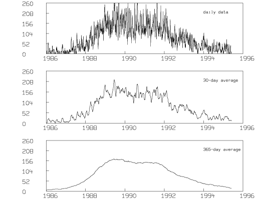
The MLAB operator MMEAN can be used to calculate moving averages of the sunspot data over periods greater than a day. For example, if the daily sunspot numbers from 1986 to 1995 are stored in the ASCII text file recssd.dat, the following MLAB commands will generate Figure 1 which shows the daily data along with month averages and year averages.
* "store AAVSO's daily data between 1986 and 1995 in a 2 column matrix"
* m4 = read(recssd,4000,2)
*
* "draw the daily data"
* draw m4
* title "daily data" at (1994,208) world size .01
* window 1986 to 1996, 0 to 260
* frame 0 to 1, .67 to 1 * w1 = w
*
* "smooth the data using moving mean operator with 30 day window"
* m2 = m4 col 1 ' mmean(m4 col 2,30)
* draw m2
* title "30-day average" at (1994,208) world size .01
* window 1986 to 1996, 0 to 260
* frame 0 to 1, .33 to .67 * w2 = w
*
* "smooth the data using moving mean operator with 365 day window" \
* m3 = m4 col 1 &' mmean(m4 col 2,365)
* draw m3
* title "365-day average" at (1994,208) world size .01
* window 1986 to 1996, 0 to 260
* frame 0 to 1, 0 to .33
*
* view

The MMEAN operator in MLAB takes a sequence of numbers and a window width and computes the average of the numbers in the window as the center of the window proceeds from the first number in the sequence to the last number in the sequence. For windows extending beyond the first or last number in the sequence, a variety of extension options are provided; the default extension method-which prepends copies of the first number to the beginning of the sequence and appends copies of the last number to the end of the sequence, as needed-was used in this example. The general effect of the moving average is to smooth noisy data. Larger windows are seen to yield smoother results.
Annual mean sunspot numbers for the years 1750 through 1994 are composed of Zurich/International and American Relative Sunspot Numbers. They are available through the CompuServe Information Service (GO SUNSPOT) and other sources. Reference 1 provides a series expansion for computing the Sun-Jupiter distance in astronomical units (1 astronomical unit = 93 million miles = 150 million kilometers) over the same period. If the Zurich data is stored in an ASCII text file called sunspots.dat and the necessary expansion coefficients from Reference 1 are stored in an ASCII text file called juprad.dat, the following MLAB commands generate Figure 2:
* "enter the AAVSO's annual averages from 1750 to 1994, make a 2"
* "column matrix with time increasing in the first column"
* m1 = read(sunspots,1000,1)
* m1 = shape(246,2,m1)
* m1 = sort(m1,1)
*
* "draw the AAVSO data"
* top title "Annual Average Sunspot Number"
* draw m1
* frame 0 to 1,.5 to 1
* w1 = w
*
* "compute Sun-Jupiter distance at Jan 1, 0:00, for each year from"
* "1750 to 1994"
* juprad = shape(244,2,0^^490)
* jrcoeff = read(juprad,53,8);
* ad1800 = jdate(1,1,1800)-.5
* fct dt(u) = (-15+32.5*(((u-ad1800)/36525)-.1)^2)/(60*60*24)
* fct vc(et) = (et-ti0)/2000
* fct f(r,t) = sum(j,0,6,jrcoeff[r,j+1]*t**j)
* k = 1;
* for i = 1750:1990:5 do {
> rw = 1+(i-1750)/5
> ti0 = jdate(1,1,jrcoeff(rw,8))-.5;
> for j = 0:4 do {
> t = jdate(1,1,i+j); "determine the Julian date of Jan. 1, year = i+j"
> v = vc(t+dt(t)); "determine the expansion's independent variable value"
> juprad[k,1] = i+j; "store the year in column 1"
> juprad[k,2] = f(rw,v); �tore the Sun-Jupiter distance in column 2"
> k = k+1;
> }
> }
*
* "draw the Sun-Jupiter distance versus time"
* top title "Sun-Jupiter distance"
* draw juprad
* frame 0 to 1, 0 to .5
* w2 = w
* view
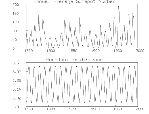
The two curves are similar in that both show about twenty three regularly spaced maxima and minima over the roughly 250 year interval.
Using the REALDFT function in MLAB, we can compute and graph the amplitude spectrum of each of the curves in Figure 2. Assuming a signal, S(t), is sampled n times and repeats with period p, it can be expanded in a Fourier series as:
|
The amplitude spectrum is then the set of points (p/j,aj) for j = 0,1,2,�,n-1. Figure 3 results from the following MLAB commands:
* "compute the amplitude spectrum of the Sun-Jupiter distance signal and"
* "annual average sunspot signal"
* p1 = realdft(m1)
* p2 = realdft(juprad)
*
* "convert frequencies to periods by taking reciprocal of FT's first column"
* "delete first rows to eliminate divide-by-zeros"
* delete p1 row 1, p2 row 1
* p1 col 1 = 1/(p1 col 1)
* p2 col 1 = 1/(p2 col 1)
*
* "draw the amplitude spectrum of the Sunspot data"
* top title "Amplitude Spectrum of Sunspot Numbers"
* draw p1 col 1:2
* frame 0 to 1, .5 to 1
* w3 = w
*
* "draw the amplitude spectrum of the Sun-Jupiter distance"
* top title "Amplitude Spectrum of Sun-Jupiter distance"
* draw p2 col 1:2
* frame 0 to 1, 0 to .5
* w4 = w
*
* blank w1,w2
* view
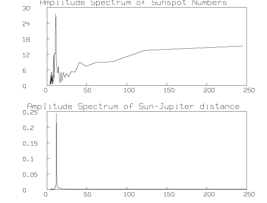
The dominant frequency component in both the annual average sunspot number data and the Sun-Jupiter distance data is seen to have a period of roughly 11 years.
If the Sun-Jupiter distance data is considered to be a periodic input function, I(t), which is transformed by some unknown periodic transfer function, T(t), to yield the annual average sunspot data as a periodic output function, S(t), by the following relation,
|
then the MLAB function DECONV can be used to estimate the unknown transfer function as follows:
* "Sun-Jupiter distance signal is the input signal and the"
* "annual average sunspot data is the output signal; compute the"
* "transfer function"
* z = deconv(juprad col 2,m1 col 2,2)
*
* "draw the transfer function with the input and output signals"
* draw (m1 col 1) &' z
* frame 0 to 1, 0 to .33
* top title "Transfer function"
* w5 = w
* blank w3,w4
* unblank w1,w2
* frame 0 to 1,.67 to 1 in w1
* frame 0 to 1,.33 to .67 in w2
* view
The resulting transfer function is shown with the input and output functions in Figure 4.
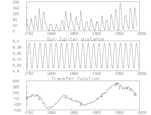
Note that the computed transfer function corresponds roughly to the modulation in amplitude of the input signal observed in the output signal. It would be interesting to research if the transfer function corresponds to some physical process occurring in the sun.
MLAB has a non-linear least squares curve fitting operation that can be used to extrapolate the sunspot data to the future. We can find values for the parameters a,b,c, and d in the function
|
which minimize
|
where (ti,y(ti)), i = 1,2,�,n are the sunspot data of interest; here we consider monthly average sunspot data from 1900 to 1985 and the yearly average sunspot data from 1750 to 1995. If an ASCII file called slm.dat contains the monthly average sunspot data from 1900 to 1985 given in the appendix of Reference 2, and the ASCII file called recssm.dat contains the monthly average sunspot data from 1985 to 1995 from AAVSO, the following MLAB commands will result in Figure 5 which shows the daily sunspot data, month average sunspot data, year average sunspot data, and extrapolated fitted curves.
* "enter Marple's monthly averages from 1900 to 1985"
* m2 = read(slm,1020,2)
* m2 = sort(m2,1)
*
* "enter AAVSO's monthly averages from 1985 to 1995 and concatenate with"
* "Marple's data"
* m3 = read(recssm,1000,2)
* m2 = m2 m3
*
* "fit to find the offset in each data set"
* fct f1(t) = d1
* d1 = 40
* fit d1, f1 to m1
final parameter values
      value 	    error	  dependency	parameter
    52.4004065 	 2.654515798 	    0 		   D1
2 iterations
CONVERGED
best weighted sum of squares = 4.246898e+005
weighted root mean square error = 4.163445e+001
weighted deviation fraction = 5.040686e-001
* fct f2(t) = d2
* d2 = 40
* fit d2, f2 to m2
final parameter values
      value 	    error	  dependency	parameter
   61.90062665   1.524683901 	     0 		   D2
2 iterations
CONVERGED
best weighted sum of squares = 2.981508e+006
weighted root mean square error = 5.132096e+001
weighted deviation fraction = 5.160940e-001
R squared = 2.342744e-015
*
* "esing the offset, fit a cosine curve to find the period in each data set"
* fct f1(t) = a1*cos(b1*(t-c1))+d1
Redefining F1
* a1 = 40; b1 = 2*pi/11; c1 = -1749;
* fit (a1,b1,c1), f1 to m1
final parameter values
      value	    error	  dependency	parameter
   29.02077265   3.269184404    4.382000966e-005   A1
   0.5695259285  0.001604153238 0.9996200793       B1
   -1759.006943  10.2264283     0.9996200791       C1
3 iterations
CONVERGED
best weighted sum of squares = 3.204926e+005
weighted root mean square error = 3.631666e+001
weighted deviation fraction = 4.226415e-001
R squared = 2.453489e-001
* fct f2(t) = a2*cos(b2*(t-c2))+d2
Redefining F2
* a2 = 40; b2 = 2*pi/11; c2 = -1900;
* fit (a2,b2,c2), f2 to m2
final parameter values
      value         error	  dependency	parameter
   56.46748013   1.36633036 	0.000234975336	   A2
   0.6012346023 0.0008759293804 0.9999436943 	   B2
   -1708.911894  5.327618133    0.9999436942	   C2
18 iterations
CONVERGED
best weighted sum of squares = 1.186679e+006
weighted root mean square error = 3.240614e+001
weighted deviation fraction = 3.232770e-001
R squared = 6.019871e-001
*
* "draw the annual averaged data with circles, the monthly averages with"
* "crosses, the fit of the annual averaged data with a solid line,"
* "and the fit of the monthly averaged data with a dashed line"
* draw m1 lt none pt circle ptsize .01 color red
* draw m2 lt none pt crosspt ptsize .01 color green
* draw m4 lt none pt dotpt color orange
* draw points(f1,1900:2010!500) lt dashed color yellow
* draw points(f2,1900:2010!500)
* window 1986 to 2006, 0 to 320
* draw 1993 ' 300 pt dotpt color orange
* draw 1993 ' 280 pt crosspt ptsize .01 color green
* draw 1993 ' 260 pt circle ptsize .01 color red
* draw (1992.5 1993.5) ' (240 240)
* draw (1992.5 1993.5) ' (220 220) lt dashed color yellow
* title "day average" at (1995,300) world size .01 color orange
* title "month average" at (1995,280) world size .01 color orange
* title "year average" at (1995,260) world size .01 color red
* title "cosine fit of month averages since 1900" at (1995,240) world size .01
* title "cosine fit of year averages since 1750" at (1995,220) world \
: size .01 color yellow
* top title "Time Variation of Sunspots"
* left title "Relative Sunspot No."
* bottom title "Year"
* view
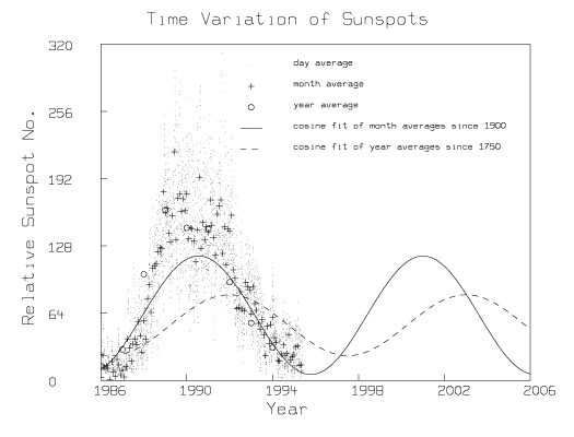
According to these simple cosine models, the next maximum in sunspot activity is to be expected between 2001 and 2003.
A visual method for finding periodic trends in annual average sunspot number data is to create a surface by stacking sunspot data between successive maxima and examining contours of constant value on the resulting surface. The following MLAB commands use the CONTOUR operator to find trends in 11 year periods of both the annual average sunspot data and the best fitting cosine model.
* "draw contour diagram of folded time series"
* cnst = 2*pi/b1; nx = 22; ny = 11;
* fct f(x,y) = lookup(m1,1750+y*cnst/ny+x*cnst)
* z1 = cross(0:21,0:10)
* z1 col 3 = f on z1
* m1 = points(f1,m1 col 1)
* z2 = z1 col 1:2
* z2 col 3 = f on z2
* mz = maxv(z2 col 3)
*
* "find contour levels for the annual averaged sunspot data and cosine model"
* cc8 = contour(z2,10:(mz-10)!4)
* cc7 = contour(z1,10:(mz-10)!4)
* draw cc7 lt 7 in w
* top title "Sunspot data"
* window 0 to 21,0 to 10*cnst/11
* xaxis 0:21:3 '0 label 1750:1981:33 labelsize .015 ffract offset(-.01,-.025) \
: ffract pt utick format(-3,5,0,0,2,0)
* yaxis 0 '(0:(cnst*10/11)!6) label 0:(cnst*10/11)!6 labelsize .015 ffract \
: offset(-.09,-.01) ffract pt rtick format(-3,5,0,0,2,0)
* frame 0 to .5, 0 to 1
* w1 = w
*
* "draw contour diagram of cosine model"
* draw cc8 lt 7 in w
* top title "Cosine model"
* window 0 to 21,0 to 10*cnst/11
* xaxis 0:21:3 '0 label 1750:1992:33 labelsize .015 ffract offset(-.01,-.025) \
: ffract pt utick format(-3,5,0,0,2,0)
* yaxis 0 '(0:(cnst*10/11)!6) label 0:(cnst*10/11)!6 labelsize .015 ffract \
: offset(-.09,-.01) ffract pt rtick format(-3,5,0,0,2,0)
* frame .5 to 1, 0 to 1
* view
The resulting graphs are shown in Figure 6.
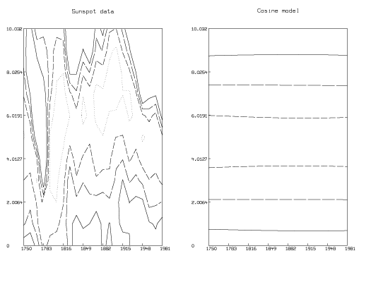
The contours in these graphs that correspond to the highest level are drawn with solid lines; those contours that correspond to the lower levels are drawn with successively shorter dashed lines; the contours corresponding to the lowest level are drawn with dotted lines. Note that each period of sunspot data is treated as a vertical slice of the composed surface.
A three dimensional perspective view of these surfaces looking down the sunspot minimum valley with time increasing as one progresses up the valley toward the point of perspective can be generated in MLAB with the following commands:
* "draw 3d perspective views of the 2 surfaces"
* blank w1,w
* draw z1 lt hidden
* cmd3d("surface zrotate 90")
* cmd3d("raise 1");
* cmd3d("track")
* cmd3d("dolly .5");
* cmd3d("box")
* cmd3d("colorlist 0,1");
* frame 0 to .5, 0 to 1 in w3
* w3d = w3
* draw z2 lt hidden
* cmd3d("surface zrotate 90")
* cmd3d("raise 1");
* cmd3d("track")
* cmd3d("dolly .5");
* cmd3d("box")
* cmd3d("colorlist 0,1");
* frame .5 to 1, 0 to 1 in w3
* view
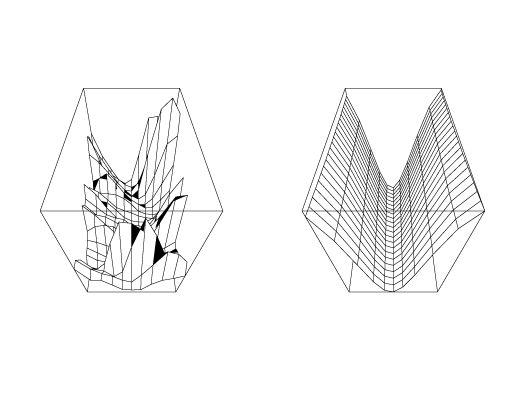
It is apparent from the contour map and 3D-perspective view that although the sunspot data follows an 11 year cycle from maximum to maximum (or minimum to minimum), there is considerable drift in the occurrence of the minimum (maximum) from one period to the next.
This paper has demonstrated some of the data analysis capabilities of MLAB within the context of sunspot number data. MLAB can be used for analyzing many other types of time-series data. For more information about what MLAB can do for your data analysis problems, please peruse the rest of our webpage.
References:
1. Pierre Bretagnon and Jean-Louis Simon. Planetary Programs and Tables from -4000 to +2800. (Richmond, VA: Willmann-Bell, Inc., 1986).
2. S. Lawrence Marple. Digital Spectral Analysis with Applications. (Inglewood Cliffs, NJ: Prentice-Hall: 1987).