Two Chemical Kinetics Models of a Laser

Two Chemical Kinetics Models of a Laser

Introduction

Since the 1950's, many devices have been discovered which produce coherent, monochromatic, electromagnetic radiation by irradiating a sample of solid, liquid, or gas that is contained in a chamber having dimensions equal to some multiple of the radiation's wavelength. Known as MASERs or LASERs, these devices can be modelled in terms of chemical reactions where photons, atoms, and molecules occupying different energy states are the reactants and products. In this paper we use the MLAB mathematical modelling program to develop chemical kinetics models of systems that amplify electromagnetic radiation by stimulated emission.

The Three State Model

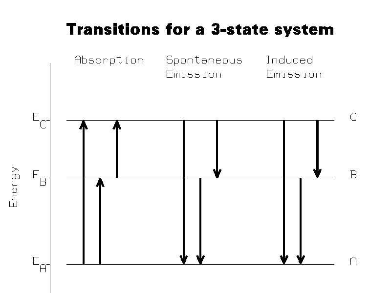
This section refers to a system of atoms which can undergo transitions between three states. Figure 1 shows the energy levels of the three-state atom, and the types of transitions that can occur between them. The states, in order of increasing energy, are designated A, B, and C. The energies of the states are designated E_A, E_B, and E_C, respectively.

Three types of reactions are seen to occur: absorption reactions, spontaneous emission reactions, and induced (also known as stimulated) emission reactions. The three spontaneous emission reactions are:

	K^s_CA
C	®	A + w_CA

	K^s_BA
B	®	A + w_BA

	K^s_CB
C	®	B + w_CB

The three absorption reactions are:

	K^a_AC
A + w_CA	®	C

	K^a_AB
A + w_BA	®	B

	K^a_BC
B + w_CB	®	C

The three induced emission reactions are:

	Kⁱ_CA
C + w_CA	®	A + 2 w_CA

	Kⁱ_CB
C + w_CB	®	B + 2 w_CB

	Kⁱ_BA
B + w_BA	®	A + 2 w_BA

In these reactions, w represents a photon; its subscript specifies its frequency. For example, w_CA is a photon with frequency (E_C-E_A)/(^h/_2p) where (^h/_2p) is Planck's constant. We use K to represent the rate constant for the reaction. The superscripts a, s, and i on K identify whether the rate constant is for an absorption, spontaneous emission, or induced emission reaction, respectively. The subscripts on K identify the reactant and product states involved in the reaction. For example Kⁱ_BA is the rate constant for the induced emission reaction in which an atom in state B reacts with a photon to produce an atom in state A and two photons.

In a collection of N three-state atoms at equilibrium, the number of atoms in the j^th atomic state is given by the Boltzmann distribution,

N_j = N(e^-E_j/kT ) / (

C
å
i=A
e^-E_i/kT)

where j is the state label A,B, or C; T is the temperature in degrees Kelvin; N is the total number of atoms in all states; and k is Boltzmann's constant. At room temperature and with the energies we are considering here, the populations of states B and C are negligible when the system is at equilibrium.

In order to generate monochromatic, electromagnetic radiation of frequency w_BC by stimulated emission, the collection of three-state atoms must get energy in the form of photons of frequency (E_C-E_A)/(^h/_2p). This pumping of the system disrupts the equilibrium distribution of states and creates a population inversion; the number of atoms in state C becomes greater than the number of atoms in state B. When this condition exists, the presence of a photon of frequency w_BC catalyzes the the transition from C to B and produces another coherent photon. If the population inversion can be maintained, significant numbers of coherent photons can be produced.

Spontaneous emission reactions follow rate laws that depend only on the number of atoms in the reactant state. Absorption and induced emission reactions follow rate laws that depend on both the number of atoms in the reactant state and the number of reactant photons. From these rules and the nine reactions listed above, we can write six coupled chemical rate equations; one for the population of each of the three states and one for the number of photons at each of the three different frequencies. Using N_A(t), N_B(t), and N_C(t) as the populations of states A, B, and C, respectively, and N_AB(t), N_BC(t), and N_AC(t) as the number of photons having frequency (E_B-E_A)/(^h/_2p), frequency (E_C-E_B)/(^h/_2p), and frequency (E_C-E_A)/(^h/_2p), respectively, the equations are:

dN_A
dt

=

-K^a_ACN_AC(t)N_A(t)-K^a_ABN_AB(t)N_A(t)+K^s_CAN_C(t)+K^s_BAN_B(t)+

Kⁱ_CAN_AC(t)N_C(t)+Kⁱ_BAN_AB(t)N_B(t)

dN_B
dt

=

-K^a_BCN_BC(t)N_B(t)+K^a_ABN_AB(t)N_A(t)+K^s_CBN_C(t)-K^s_BAN_B(t)+

Kⁱ_CBN_BC(t)N_C(t)-Kⁱ_BAN_AB(t)N_B(t)

dN_C
dt

=

- dN_A
dt
- dN_B
dt

dN_AB
dt

=

-k^a_AB N_AB(t) N_A(t)+k^s_BA N_B(t)+kⁱ_BA N_AB(t) N_B(t)-k^d_AB N_AB(t)

dN_AC
dt

=

pump_AC(t)-k^a_AC N_AC(t) N_A(t)+k^s_CA N_C(t)+kⁱ_CA N_AC(t) N_C(t)-k^d_AC N_AC(t)

dN_BC
dt

=

-k^a_BC N_BC(t) N_B(t)+k^s_CB N_C(t)+kⁱ_CB N_BC(t) N_C(t)-k^d_BC N_BC(t)

The function pump_AC(t) represents the number of photons per second that are put into the system to pump the ground state A atoms to the state C. The terms k^d_AB N_AB(t) and k^d_ACN_AC(t) represent the number of photons per second that are lost due to destructive interference in the chamber and the term k^d_BCN_BC(t) represents the number of w_BC photons per second that escape from the chamber.

Using MLAB, we can assign values to the different rate constants, compute the initial Boltzmann distribution of states, define the rate equations, and integrate the rate equations for a continuous wave (CW) laser by executing a script containing the following commands (comments are delimited by "/*" and "*/"):

* assign values for constants */ 
k = 1.3806E-16 /* Boltzmann's constant in erg/degree Kelvin */ 
h = 6.6261E-27 /* Planck's constant in erg sec */ 
EA = 0.1E-11 /* energy of state A in ergs */ 
EB = 1.05E-11 /* energy of state B in ergs */ 
EC = 1.06E-11 /* energy of state C in ergs */ 
N = 1000 /* total number of A,B,C, state atoms */ 
Np = 10^10 /* total number of photons per second pumped into system */ 
tmp = 293 /* initial temperature in degrees Kelvin */ 
kaAB = 1.1e7 /* A->B absorption rate constant in 1/(second*photon) */ 
kaBC = 1.1e7 /* B->C absorption rate constant in 1/(second*photon) */ 
kaAC = 1.1e7 /* A->C absorption rate constant in 1/(second*photon) */ 
ksCA = 1.1e7 /* C->A spontaneous emission rate constant in 1/second */ 
ksCB = 1.1e7 /* C->B spontaneous emission rate constant in 1/second */ 
ksBA = 1.1e7 /* B->A spontaneous emission rate constant in 1/second */ 
kiCA = .1e7 /* C->A induced emission rate constant in 1/(second*atom) */ 
kiCB = .2e7 /* C->B induced emission rate constant in 1/(second*atom) */ 
kiBA = .3e7 /* B->A induced emission rate constant in 1/(second*atom) */ 
kdAB = 1e9 /* B->A photon loss from chamber in 1/second */ 
kdBC = 1e7 /* C->B photon loss from chamber in 1/second */ 
kdAC = 1e9 /* C->A photon loss from chamber in 1/second */

/* initial A,B, and C populations from Boltzmann distribution */ 

fct g(e) = exp(-e/(k*tmp)) 
bf = g(EA)+g(EB)+g(EC) 
init NA(0) = N*g(EA)/bf /* atoms */ 
init NB(0) = N*g(EB)/bf /* atoms */ 
init NC(0) = N*g(EC)/bf /* atoms */

/* initial BA, CB, and CA numbers of photons */ 

init NAB(0) = 0 /* photons */ 
init NBC(0) = 0 /* photons */ 
init NAC(0) = 0 /* photons */

/* photon rate due to pumping A->C transition */ 
fct pumpAC(t) = Np /* photons/second */

/* rate equations */ 

fct NA't(t) = -kaAC*NAC(t)*NA(t)-kaAB*NAB(t)*NA(t)+ksCA*NC(t)  
	      +ksBA*NB(t)+kiCA*NAC(t)*NC(t)+kiBA*NAB(t)*NB(t)

fct NB't(t) = -kaBC*NBC(t)*NB(t)+kaAB*NAB(t)*NA(t)+ksCB*NC(t)  
	      -ksBA*NB(t)-kiBA*NAB(t)*NB(t)+kiCB*NBC(t)*NC(t)

fct NC't(t) = -NA't(t)-NB't(t)

fct NAB't(t) = -kaAB*NAB(t)*NA(t)+ksBA*NB(t)+kiBA*NAB(t)*NB(t)-kdAB*NAB(t)

fct NAC't(t) = pumpAC(t)-kaAC*NAC(t)*NA(t)+ksCA*NC(t)+kiCA*NAC(t)*NC(t)  
	       -kdAC*NAC(t)

fct NBC't(t) = -kaBC*NBC(t)*NB(t)+ksCB*NC(t)+kiCB*NBC(t)*NC(t)-kdBC*NBC(t)

/* integrate the kinetics equations for 1 microsecond */ 
p = integrate(NA,NB,NC,NAC,NBC,NAB,0:.000001!250) 
/* columns of p are t NA NA' NB NB' NC NC' NAC NAC' NBC NBC' NAB NAB' */

Here the number of atoms, number of photons, and rate constants have been conveniently chosen so that population inversions are achieved in the allotted time scale. The time dependent population levels of each state and the number of photons at each frequency are graphed by the following commands:

/* draw the time dependence of the number of A's, B's, and C's */ 
draw p col 1:2 
draw p col (1,4) color green 
draw p col (1,6) color red 
no framebox 
top title "population vs. time for CW laser" 
title t1 = "N'1DA'1U(t)" at (.8,.275) ffract size .01 
title t2 = "N'1DB'1U(t)" at (.8,.19) ffract color green size .01 
title t3 = "N'1DC'1U(t)" at (.8,.7) ffract color red size .01 
frame 0 to 1, .5 to 1 
w1=w

draw p col (1,8) 
draw p col (1,10) color green 
draw p col (1,12) color red 
no framebox 
top title "photons vs. time for CW laser" 
title t5 = "N'1DAC'1U(t)" at (.8,.25) ffract size .01 
title t6 = "N'1DBC'1U(t)" at (.8,.75) ffract color green size .01 
title t7 = "N'1DAB'1U(t)" at (.85,.16) ffract color red size .01 
frame 0 to 1, 0 to .5 
view

Figure 2 shows the resulting graph.

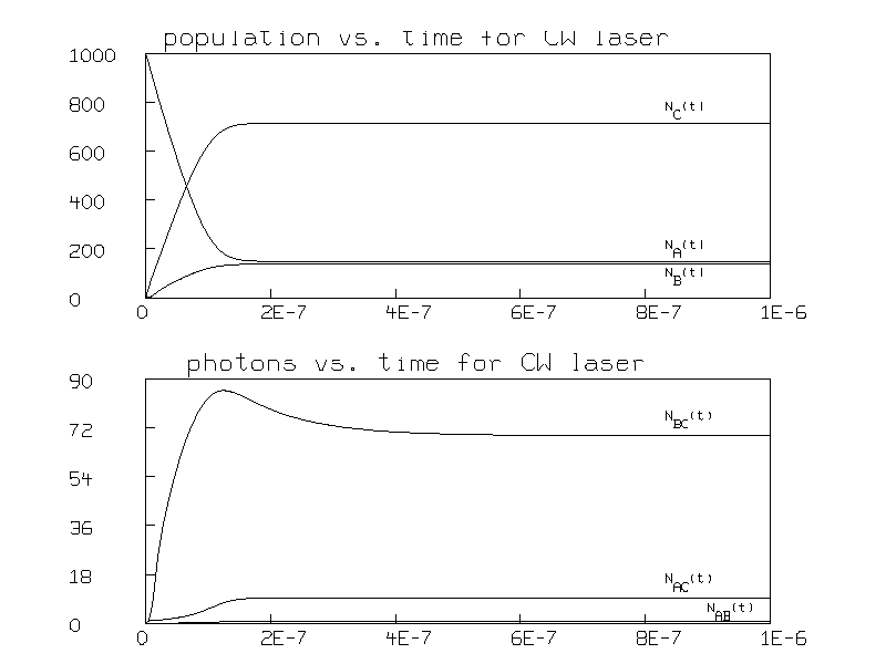
Note that the populations reach steady state after 4 ×10^-7 seconds and that the steady state populations are then greater for state C than state B; this is the expected population inversion in a laser.

The MLAB commands above model a laser that operates in a continuous mode; the pump function is constant in time. We can model a pulsed laser by using the previous MLAB commands but with the following definition of the pumping function:

/* define the pulsed input pump function */ 
fct pumpAC(t) = if (t*10000000-floor(t*10000000) < .5) then 10^10 else 0

This effectively modulates the input so that the pump alternates between 0 and 1 ×10¹⁰ photons per second 10⁷ times a second. The resulting populations and numbers of photons are graphed in Figure 3.

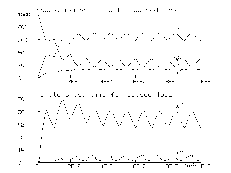
In this figure, the population inversion is seen to be modulated at the frequency of the pump pulses.

An important feature of this three-state model is that one can easily investigate how the population levels change with variations in any of the input constants: N, Np, T, K^a_AB, K^a_BC, K^a_AC, K^s_CA, K^s_CB, K^s_BA, Kⁱ_CA, Kⁱ_CB, Kⁱ_BA, K^d_AB, K^d_BC, and K^d_AC. This makes the model given above an important pedagogical tool.

The Atomic Hydrogen Laser

Another model is based on the lowest 10 levels of basic hydrogen. By the lowest 10 energy levels of basic hydrogen, we mean the 1s, 2s, 2p, 3s, 3p, 3d, 4s, 4p, 4d, and 4f levels one learns about in beginning and intermediate chemistry and physics courses. Note, this is not a hydrogen MASER, which operates on the two hyperfine levels of the 1s state. Hydrogen MASERs have been known experimentally since the late 1950's and are described in Reference 1.

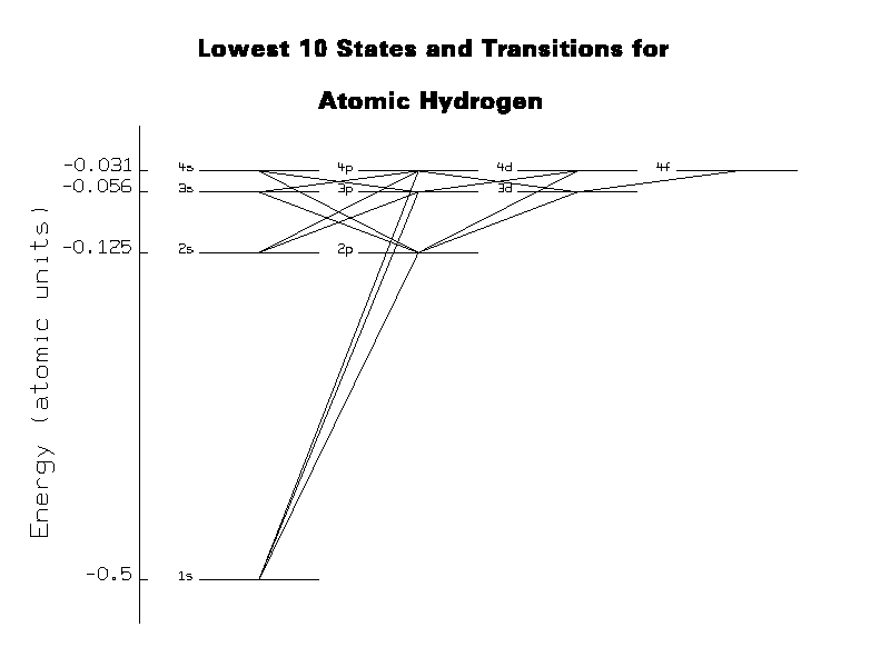
Figure 4 shows the lowest 10 levels of atomic hydrogen and the transitions that are allowed by dipole selection rules. Each line connecting two states represents three reactions: an absorption reaction, a spontaneous emission reaction, and an induced emission reaction.

The spontaneous emission rate constants for this system are calculated exactly from equations (59.11), (63.1), (63.2), and (63.3) of Reference 2. The absorption and induced emission rate constants are calculated from the values of the spontaneous emission rate constants and equations (8.5-1), (8.5-9), and (8.5-10) of Reference 3.

In this computational model, we assume only the ground state is initially populated (Boltzmann factors are not computed); and we continuously pump the 1s ® 4p transition. The decay rate constants, number of photons, and number of atoms, are conveniently selected so that lasing occurs at a frequency of (E₄-E₃)/(^h/_2p). Here are the MLAB commands:

/* assign values for constants */ 
hb = 1.0546E-27 /* Planck's constant divided by 2 pi in erg sec */ 
c = 2.9979E10 /* speed of light in vacuum (cm/sec)*/ 
ep = 4.8029E-10 /* proton charge in esu */ 
em = 9.1096E-28 /* mass of electron in grams */ 
a0 = 5.2917E-9 /* radius of 1st Bohr orbit in cm */ 
Z = 1 /* nuclear charge of hydrogen atom */ 
epau = 4.360E-11 /* ergs per atomic unit of energy */ 
N = 1e3 /* total number of atoms */ 
Np = 1e10 /* total number photons per second pumped */ 
mlt = 1E-15 /* volume proportionality constant relating spontaneous to induced processes */

/* function for evaluating energy of n-th atomic level in ergs */ 
fct E(n) = -epau*(Z^2)/(2*(n^2))

/* function for evaluating the degeneracy of state with l-orbital angular momentum */ 
fct g(l) = 2*l+1

/* functions for evaluating spontaneous emission rate constants */ 
fct f(a,b,c,d) = fact(c-a-b-1)*fact(c-1)*sum(k,max(0,1-c),min(-a,-b),       
    hgeomd(k,-a,c-a-b-1,-b)*d^k)/(fact(c-b-1)*fact(c-a-1)) 
fct R(n1,n2,l) = (-1)^(n1-l)*sqrt(fact(n2+l)*fact(n1+l-1))*(4*n1*n2)^(l+1)*\            
     (n2-n1)^(n2+n1-2*l-2)*(f(-n2+l+1,-n1+l,2*l,-4*n2*n1/(n2-n1)^2)-\
     (((n2-n1)/(n2+n1))^2)*f(-n2+l-1,-n1+l,2*l,-4*n2*n1/(n2-n1)^2))/\      
     ((4*fact(2*l-1))*sqrt(fact(n2-l-1)*fact(n1-l))*(n2+n1)^(n2+n1))
fct ks(ni,li,nf,lf) = 4*ep^2*((E(ni)-E(nf))/hb)^3*\
     ((a0*(if (lf>li) then R(ni,nf,lf) else R(nf,ni,li)))^2)/(3*hb*g(li)*c^3)

/* spontaneous emission rate constants */
ks2p1s = ks(2,1,1,0); ks3p1s = ks(3,1,1,0); ks4p1s = ks(4,1,1,0) 
ks3p2s = ks(3,1,2,0); ks4p2s = ks(4,1,2,0); ks4p3s = ks(4,1,3,0) 
ks3s2p = ks(3,0,2,1); ks4s2p = ks(4,0,2,1); ks4s3p = ks(4,0,3,1)
ks3d2p = ks(3,2,2,1); ks4d2p = ks(4,2,2,1); ks4d3p = ks(4,2,3,1) 
ks4p3d = ks(4,1,3,2); ks4f3d = ks(4,3,3,2)

/* induced emission rate constants */ 
pch = mlt*PI^2*c^3*hb^2 
ki2p1s = pch*ks2p1s/(E(2)-E(1))^3; ki3p1s = pch*ks3p1s/(E(3)-E(1))^3 
ki4p1s = pch*ks4p1s/(E(4)-E(1))^3; ki3p2s = pch*ks3p2s/(E(3)-E(2))^3 
ki4p2s = pch*ks4p2s/(E(4)-E(2))^3; ki4p3s = pch*ks4p3s/(E(4)-E(3))^3 
ki3s2p = pch*ks3s2p/(E(3)-E(2))^3; ki4s2p = pch*ks4s2p/(E(4)-E(2))^3 
ki4s3p = pch*ks4s3p/(E(4)-E(3))^3; ki3d2p = pch*ks3d2p/(E(3)-E(2))^3 
ki4d2p = pch*ks4d2p/(E(4)-E(2))^3; ki4d3p = pch*ks4d3p/(E(4)-E(3))^3 
ki4p3d = pch*ks4p3d/(E(4)-E(3))^3; ki4f3d = pch*ks4f3d/(E(4)-E(3))^3

/* absorption rate constants */ 
ka1s2p = ki2p1s*g(1)/g(0); ka1s3p = ki3p1s*g(1)/g(0) 
ka1s4p = ki4p1s*g(1)/g(0); ka2s3p = ki3p2s*g(1)/g(0) 
ka2s4p = ki4p2s*g(1)/g(0); ka3s4p = ki4p3s*g(1)/g(0) 
ka2p3s = ki3s2p*g(0)/g(1); ka2p4s = ki4s2p*g(0)/g(1) 
ka3p4s = ki4s3p*g(0)/g(1); ka2p3d = ki3d2p*g(2)/g(1) 
ka2p4d = ki4d2p*g(2)/g(1); ka3p4d = ki4d3p*g(2)/g(1) 
ka3d4p = ki4p3d*g(1)/g(2); ka3d4f = ki4f3d*g(3)/g(2)

/* decay rate constants */ 
kd12 = 1e12 /* 1<->2 photon loss from resonator in 1/second */ 
kd13 = 1e12 /* 1<->3 photon loss from resonator in 1/second */ 
kd14 = 1e12 /* 1<->4 photon loss from resonator in 1/second */ 
kd23 = 1e12 /* 2<->3 photon loss from resonator in 1/second */ 
kd24 = 1e12 /* 2<->4 photon loss from resonator in 1/second */ 
kd34 = 1e4 /* 3<->4 photon loss from resonator in 1/second */

/* initial 1s,2s,2p,3s,3p,3d,4s,4p,4d, and 4f populations */ 
init N1s(0) = N; init N2s(0) = 0; init N2p(0) = 0 
init N3s(0) = 0; init N3p(0) = 0; init N3d(0) = 0 
init N4s(0) = 0; init N4p(0) = 0; init N4d(0) = 0 
init N4f(0) = 0

/* initial 1<->2, 1<->3, 1<->4, 2<->3, 2<->4, and 3<->4 photons */ 
init N12(0) = 0; init N13(0) = 0; init N14(0) = 0 
init N23(0) = 0; init N24(0) = 0; init N34(0) = 0

/* photon rate due to pumping A->C transition */ 
fct pump14(t) = Np /* photons/second */\
   *(if t<0 then 0 else (1-(gaussd(t,0,1e-9)/gaussd(0,0,1e-9))))

/* define the rate equations */ 
fct N1s't(t) = -ka1s2p*N1s*N12-ka1s3p*N1s*N13-ka1s4p*N1s*N14  
	       +ki2p1s*N2p*N12+ki3p1s*N3p*N13+ki4p1s*N4p*N14  
               +ks2p1s*N2p +ks3p1s*N3p       +ks4p1s*N4p 
fct N2s't(t) = -ka2s3p*N2s*N23-ka2s4p*N2s*N24  
               +ki3p2s*N3p*N23+ki4p2s*N4p*N24  
               +ks3p2s*N3p    +ks4p2s*N4p 
fct N2p't(t) = +ka1s2p*N1s*N12-ka2p3s*N2p*N23-ka2p4s*N2p*N24  
               -ka2p3d*N2p*N23-ka2p4d*N2p*N24  
               -ki2p1s*N2p*N12+ki3s2p*N3s*N23+ki4s2p*N4s*N24  
               +ki3d2p*N3d*N23+ki4d2p*N4d*N24  
               -ks2p1s*N2p    +ks3s2p*N3s 
               +ks4s2p*N4s  
               +ks3d2p*N3d    +ks4d2p*N4d 
fct N3s't(t) = +ka2p3s*N2p*N23-ka3s4p*N3s*N34  
               -ki3s2p*N3s*N23+ki4p3s*N4p*N34  
               -ks3s2p*N3s     +ks4p3s*N4p 
fct N3p't(t) = +ka1s3p*N1s*N13+ka2s3p*N2s*N23-ka3p4s*N3p*N34-ka3p4d*N3p*N34                 
               -ki3p1s*N3p*N13-ki3p2s*N3p*N23+ki4s3p*N4s*N34+ki4d3p*N4d*N34  
               -ks3p1s*N3p    -ks3p2s*N3p    +ks4s3p*N4s    +ks4d3p*N4d 
fct N3d't(t) = +ka2p3d*N2p*N23-ka3d4p*N3d*N34-ka3d4f*N3d*N34  
               -ki3d2p*N3d*N23+ki4p3d*N4p*N34+ki4f3d*N4f*N34  
               -ks3d2p*N3d    +ks4p3d*N4p    +ks4f3d*N4f 
fct N4s't(t) = +ka2p4s*N2p*N24+ka3p4s*N3p*N34  
               -ki4s2p*N4s*N24-ki4s3p*N4s*N34  
               -ks4s2p*N4s    -ks4s3p*N4s 
fct N4p't(t) = +ka1s4p*N1s*N14+ka2s4p*N2s*N24+ka3s4p*N3s*N34+ka3d4p*N3d*N34                 
               -ki4p1s*N4p*N14-ki4p2s*N4p*N24-ki4p3s*N4p*N34-ki4p3d*N4p*N34  
               -ks4p1s*N4p    -ks4p2s*N4p    -ks4p3s*N4p    -ks4p3d*N4p 
fct N4d't(t) = +ka2p4d*N2p*N24+ka3p4d*N3p*N34  
               -ki4d2p*N4d*N24-ki4d3p*N4d*N34  
               -ks4d2p*N4d    -ks4d3p*N4d 
fct N4f't(t) = +ka3d4f*N3d*N34-ki4f3d*N4f*N34-ks4f3d*N4f 
fct N12't(t) = -ka1s2p*N1s*N12+ki2p1s*N2p*N12+ks2p1s*N2p-kd12*N12 
fct N13't(t) = -ka1s3p*N1s*N13+ki3p1s*N3p*N13+ks3p1s*N3p-kd13*N13 
fct N14't(t) = pump14(t)-ka1s4p*N1s*N14+ki4p1s*N4p*N14+ks4p1s*N4p-kd14*N14 
fct N23't(t) = -ka2s3p*N2s*N23+ki3p2s*N3p*N23+ks3p2s*N3p  
               -ka2p3s*N2p*N23+ki3s2p*N3s*N23+ks3s2p*N3s  
               -ka2p3d*N2p*N23+ki3d2p*N3d*N23+ks3d2p*N3d-kd23*N23 
fct N24't(t) = -ka2s4p*N2p*N24+ki4p2s*N4p*N24*ks4p2s*N4p  
               -ka2p4s*N2p*N24+ki4s2p*N4s*N24+ks4s2p*N4s  
               -ka2p4d*N2p*N24+ki4d2p*N4d*N24+ks4d2p*N4d-kd24*N24 
fct N34't(t) = -ka3s4p*N3s*N34+ki4p3s*N4p*N34+ks4p3s*N4p 
               -ka3p4s*N3p*N34+ki4s3p*N4s*N34+ks4s3p*N4s  
               -ka3p4d*N3p*N34+ki4d3p*N4d*N34+ks4d3p*N4d  
               -ka3d4p*N3d*N34+ki4p3d*N4p*N34+ks4p3d*N4p  
               -ka3d4f*N3d*N34+ki4f3d*N4f*N34+ks4f3d*N4f-kd34*N34

/* integrate the kinetics equations for .001 seconds */ 
disastersw = -1 
p = integrate(N1s,N2s,N2p,N3s,N3p,N3d,N4s,N4p,N4d,N4f,N12,N13,N14,N23,N24,  N34,0:.001!250) 
/* cols  p: T  N1s  N1s'T  N2s  N2s'T  N2p  N2p'T  N3s  N3s'T 
               N3p  N3p'T  N3d  N3d'T  N4s  N4s'T  N4p  N4p'T 
               N4d  N4d'T  N4f  N4f'T  N12  N12'T  N13  N13'T 
               N14  N14'T  N23  N23'T  N24  N24'T  N34  N34'T */

Here is the graph of the total populations of the N=4 and N=3 levels versus time:

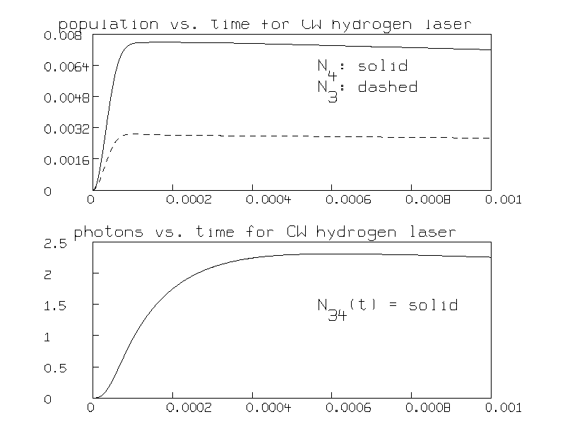
The population inversion is seen to occur after .0005 seconds.

Mathematical models of molecular lasers can be implemented in a manner similar to that used here to model an atomic laser. Additional terms in the rate equations may be introduced that account for various radiationless relaxation processes, such as rotational-to-vibrational relaxation and electronic-to-vibrational relaxation. A computational limitation does arise in such mathematical models when there are many coupled rate equations; the equations become difficult to integrate without numerical errors accruing at each time step. Such systems of equations are referred to as ill-conditioned and one can see erroneous exponential growth in one or more of the quantities of interest. Although MLAB employs several ordinary differential equation-solving algorithms, including Gear's method for integrating stiff equations, solving ill-conditioned differential equations over too large an interval will produce unreliable results.

References

1. Norman F. Ramsey, ``The Atomic Hydrogen Maser'', American Scientist 56 (1968) 420-438.

2. Hans A. Bethe and Edwin E. Salpeter, Quantum Mechanics of One- and Two-Electron Atoms (NY: Plenum Publishing Corp, 1977) 248-269.

3. Amnon Yariv, Quantum Electronics (NY: John Wiley and Sons, 1989) 171-173.